
Numpy Reloaded#

Unless specified differently, these slides are copyright CINECA 2019 and are released under the Attribution--NonCommercial--NoDerivs (CC BY-NC-ND) Creative Commons license, version 3.0. Uses not allowed by the above license need explicit, written permission from the copyright owner. For more information see: http://creativecommons.org/licenses/by-nc-nd/3.0/
Slides were authored by Sergio Orlandini.
import numpy as np

import matplotlib.pyplot as plt
from mpl_toolkits.mplot3d import Axes3D

def plot_order(order='C'):
    """function to plot order figures"""

    row, col = 3, 4

    fig = plt.figure(figsize=(15,10))
    gs = fig.add_gridspec(1, 3)

    ax = [None] * 2
    ax[0] = fig.add_subplot(gs[0, 0])
    ax[1] = fig.add_subplot(gs[0, 1:])

    a = np.empty((row, col), order=order)

    if np.isfortran(a):
        for i in np.arange(col):
            a[:,i]  = - i*row*3 - np.arange(0, row)
        b = a.T
    else:
        for i in np.arange(row):
            a[i,:]  = - i*col*3 - np.arange(0, col)
        b = np.copy(a)

    b += 100
    b.shape = (1, col*row)

    cmap = plt.cm.plasma
    for axis, array in zip(ax, [a, b]):
        axis.matshow(array, cmap=cmap)
        axis.set_xticks([], [])
        axis.set_yticks([], [])

    for j in np.arange(row):
        for i in np.arange(col):
            ax[0].text(i, j, f"{j},{i}", va='center', ha='center', fontsize=16)

    plt.subplots_adjust(wspace=0.4)
    plt.show()


def graph(a, b, c):
    """function to plot broadcasting figures"""
    if not hasattr(b, 'shape'): b = np.array([b])
    if b.ndim == 1: b.shape = (1, b.shape[0])

    a, b, c = a.shape, b.shape, c.shape

    offset = 1
    dim = a[1] * 3 + 3 * offset
    index = np.indices((dim, dim, dim))

    def slice_cube(orig, size):
        r = np.full(index[0].shape, True) & (index[1] < 1)
        for i, d in enumerate([0, 2]):
            r &= (index[d] >= orig[i]) & (index[d] < orig[i] + size[(i+1)%2])
        return r

    fig = plt.figure(figsize=(10,8))
    #ax = fig.gca(projection='3d', azim=-75, elev=20)
    ax = fig.add_subplot(projection='3d', azim=-75, elev=20)
    plt.axis('off')
    plt.margins(0,0,0)
    ax.set_xlim([0, dim]); ax.set_ylim([0, dim/2]); ax.set_zlim([-0.5, dim])

    cubes = [None] * 4
    # 1st cube
    orig = np.zeros(2, dtype=int)
    cubes[0] = slice_cube(orig, a)
    ax.text(orig[0]+a[1]/1.5, 0, -1.5, str(a), ha='center', fontsize=16)
    # 2nd expansion cube
    orig[0] += a[1] + offset
    cubes[1] = slice_cube(orig, c)
    ax.text(orig[0]+c[1]/1.5, 0, -1.5, str(b), ha='center', fontsize=16)
    # 2nd cube
    cubes[2] = slice_cube(orig, b)
    # 3rd cube
    orig[0] += c[1] + offset * 2
    cubes[3] = slice_cube(orig, c)
    ax.text(orig[0]+c[1]/1.5, 0, -1.5, str(c), ha='center', fontsize=16)

    voxels = np.full_like(cubes[0], False)
    for i in cubes:
        voxels |= i

    cname = ['red', 'white', 'red', 'cornflowerblue']
    colors = np.empty(voxels.shape, dtype=object)
    for i, c in enumerate(cubes):
        colors[c] = cname[i%len(cubes)]

    ax.voxels(voxels, facecolors=colors, edgecolor='k', alpha=0.8)
    ax.invert_zaxis()
    plt.tight_layout()
    plt.show()
Broadcast#
Numpy array ufunc operations are performed element-wise.
In principle element-by-element arithmetic operations can be performed only between arrays of same shape.
Instead Numpy has a mechanism to perform arithmetic operations between arrays of different shape.
The capability to operate with array of different shape is called broadcasting,
because the smaller array is broadcasted in order to fulfill larger arrays.
A very simple example is the arithmetic operations between arrays and scalars
x = np.arange(10)
x
array([0, 1, 2, 3, 4, 5, 6, 7, 8, 9])
x + 42
array([42, 43, 44, 45, 46, 47, 48, 49, 50, 51])
In this case the scalar is extended until the same dimension of the array is reached.
Of course all the process is performed in an efficient way and no copies or replicas are needed.
Broadcasting is not always allowed but it is subject to constrains and follow some rules.
First of all for Numpy two dimension2 are comparable when:
equals
one of them is 1
A ufunc operation is allowed only between arrays with comparable dimensions.
Broadcasting rules:
In the case of arrays with different dimensions, the shape of smaller array is increased from the leading dimension (starting from the left) with 1
If the shape in any dimension is different but comparable the array with shape equal to 1 is stretched along this direction in order to match the shape of larger array
At this point the opeartion can be performed element-wise
The shape of the resulting array is the maximum size along each dimension of the input arrays.
If at least one of the dimension is not comparable, the array shapes are not compatible, and an error of type ValueError: frames are not aligned exception is thrown is raised
x = np.arange(6).reshape(2, 3)
y = 42

x.shape
(2, 3)
x  | 2 x 3 | 2 x 3 |
y  |     1 | 1 x 1 |
             -----
output       2 x 3
x + y
array([[42, 43, 44],
       [45, 46, 47]])
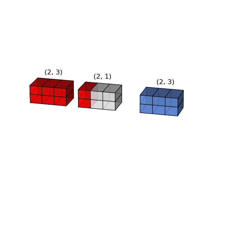
graph(x, y, x+y)

x = np.arange(6).reshape(2, 3)
y = np.arange(2).reshape(2, 1)
x  | 2 x 3
y  | 2 x 1
     -----
out  2 x 3
(x + y).shape
(2, 3)
graph(x, y, x+y)
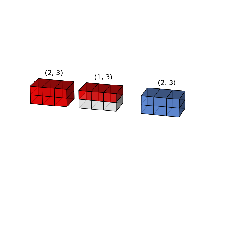
x = np.arange(6).reshape(2, 3)
y = np.arange(3)
x  | 2 x 3 | 2 x 3 |
y  |     3 | 1 x 3 |
             -----
output       2 x 3
(x + y).shape
(2, 3)
graph(x, y, x+y)
x = np.arange(6).reshape(3, 2)
y = np.arange(3)
x  | 3 x 2 | 3 x 2 |
y  |     3 | 1 x 3 |
             -----
output       ? ? ?
>>> x + y
ValueError: operands could not be broadcast together with shapes (3,2) (3,)
x = np.arange(4).reshape(4, 1)
y = np.arange(1).reshape(1, 1)

graph(x , y, x+y)

x = np.arange(4).reshape(1, 4)
y = np.arange(1).reshape(1, 1)

graph(x, y, x+y)

Broadcasting can be useful to perform outer product of arrays
x = np.arange(1, 11).reshape(10, 1)
y = np.arange(1, 11).reshape(1, 10)

x, y
(array([[ 1],
        [ 2],
        [ 3],
        [ 4],
        [ 5],
        [ 6],
        [ 7],
        [ 8],
        [ 9],
        [10]]),
 array([[ 1,  2,  3,  4,  5,  6,  7,  8,  9, 10]]))
x * y
array([[  1,   2,   3,   4,   5,   6,   7,   8,   9,  10],
       [  2,   4,   6,   8,  10,  12,  14,  16,  18,  20],
       [  3,   6,   9,  12,  15,  18,  21,  24,  27,  30],
       [  4,   8,  12,  16,  20,  24,  28,  32,  36,  40],
       [  5,  10,  15,  20,  25,  30,  35,  40,  45,  50],
       [  6,  12,  18,  24,  30,  36,  42,  48,  54,  60],
       [  7,  14,  21,  28,  35,  42,  49,  56,  63,  70],
       [  8,  16,  24,  32,  40,  48,  56,  64,  72,  80],
       [  9,  18,  27,  36,  45,  54,  63,  72,  81,  90],
       [ 10,  20,  30,  40,  50,  60,  70,  80,  90, 100]])
Put in order a Numpy Array#
A Numpy array is a contiguous segment of memory with an indexing scheme.
For one-dimensional array there is a unique indexing scheme but for a two or more dimensional arrays there are two indexing scheme.
Indeed in a 1D segment of memory data can be stored in row-major or column-major order.
In row-major order the elements of a row are close in memory (C-style),
it means that the row indices vary the slowest, and the column indices the quickest.
While in column-major order the elements are stored by columns (Fortran-style).

What is the indexing order of a Numpy Array?#
np.arange(12).reshape((3, 4))
array([[ 0,  1,  2,  3],
       [ 4,  5,  6,  7],
       [ 8,  9, 10, 11]])
%matplotlib inline
import matplotlib.pyplot as plt

plot_order("C")
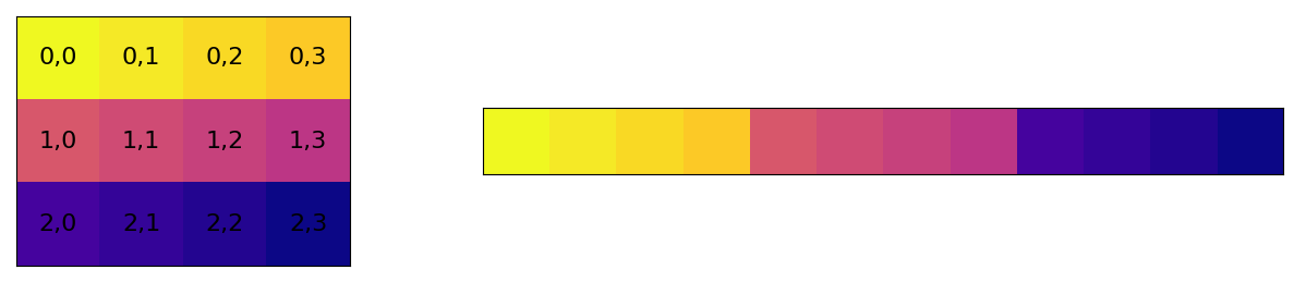
Numpy support any order of indices, both row-major and column-major. The default is row-major ordering or C-style.
When executing ufunc Numpy is smart to determine the fastest index for efficient memory access in innermost loop accordingly to array ordering.
c = np.arange(12).reshape((3, 4), order='c') # default
c
array([[ 0,  1,  2,  3],
       [ 4,  5,  6,  7],
       [ 8,  9, 10, 11]])
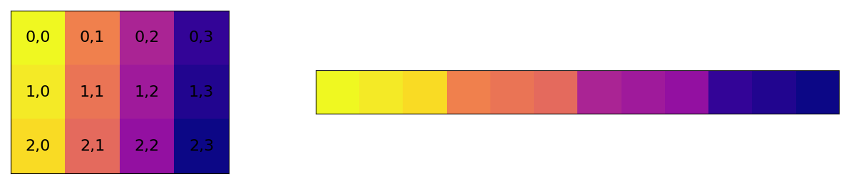
f = np.arange(12).reshape((3, 4), order='f')
f
array([[ 0,  3,  6,  9],
       [ 1,  4,  7, 10],
       [ 2,  5,  8, 11]])
plot_order("F")
c.flags
  C_CONTIGUOUS : True
  F_CONTIGUOUS : False
  OWNDATA : False
  WRITEABLE : True
  ALIGNED : True
  WRITEBACKIFCOPY : False
  UPDATEIFCOPY : False
f.flags
  C_CONTIGUOUS : False
  F_CONTIGUOUS : True
  OWNDATA : False
  WRITEABLE : True
  ALIGNED : True
  WRITEBACKIFCOPY : False
  UPDATEIFCOPY : False
np.arange(42).flags
  C_CONTIGUOUS : True
  F_CONTIGUOUS : True
  OWNDATA : True
  WRITEABLE : True
  ALIGNED : True
  WRITEBACKIFCOPY : False
  UPDATEIFCOPY : False
np.array
array(object, dtype=None, copy=True, order='K', subok=False, ndmin=0)

    Create an array.
...
    order : {'K', 'A', 'C', 'F'}, optional
        Specify the memory layout of the array. If object is not an array, the
        newly created array will be in C order (row major) unless 'F' is
        specified, in which case it will be in Fortran order (column major).
        If object is an array the following holds.

        ===== ========= ===================================================
        order  no copy                     copy=True
        ===== ========= ===================================================
        'K'   unchanged F & C order preserved, otherwise most similar order
        'A'   unchanged F order if input is F and not C, otherwise C order
        'C'   C order   C order
        'F'   F order   F order
        ===== ========= ===================================================
...
c = np.array([[3.14, 2.718, 1.618], [6.022*10**23, 299792, 1.3806*10**-23], [42, 101010, 0x2A]], order='C')
c
array([[3.14000e+00, 2.71800e+00, 1.61800e+00],
       [6.02200e+23, 2.99792e+05, 1.38060e-23],
       [4.20000e+01, 1.01010e+05, 4.20000e+01]])
f = np.array([[3.14, 2.718, 1.618], [6.022*10**23, 299792, 1.3806*10**-23], [42, 101010, 0x2A]], order='F')
f
array([[3.14000e+00, 2.71800e+00, 1.61800e+00],
       [6.02200e+23, 2.99792e+05, 1.38060e-23],
       [4.20000e+01, 1.01010e+05, 4.20000e+01]])
c[1, 2]
1.3806e-23
f[1, 2]
1.3806e-23
np.array_equal(c, f)
True
Can memory layout affect the performance?#
n = 1000000

x = np.arange(n)

%time _ = x.sum()
CPU times: user 1.35 ms, sys: 146 µs, total: 1.5 ms
Wall time: 1.44 ms
stride = 65

x = np.arange(n*stride)[::stride]

%time _ = x.sum()
CPU times: user 20.2 ms, sys: 0 ns, total: 20.2 ms
Wall time: 20.2 ms
Iterate over Arrays#
x = np.arange(12).reshape(3, 4)
x
array([[ 0,  1,  2,  3],
       [ 4,  5,  6,  7],
       [ 8,  9, 10, 11]])
manually iterate over arrays
for i in np.arange(x.shape[0]):
    for j in np.arange(x.shape[1]):
        print(x[i,j], end=', ')
0, 1, 2, 3, 4, 5, 6, 7, 8, 9, 10, 11,
default iterator iterate over last dimension
for i in x:
    print(i, end=', ')
[0 1 2 3], [4 5 6 7], [ 8 9 10 11],
In Numpy there is an iterator object np.nditer.
It is an efficient multi-dimensional iterator with which it is possible to iterate over an array
for i in np.nditer(x):
    print(i, end=', ')
0, 1, 2, 3, 4, 5, 6, 7, 8, 9, 10, 11,
NB:
The order of iterations reflects the ordering of the data in memory.
This is due to efficiency reasons considering the fact that
the order of the iterations is not important but only the fact that all the elements are visited.
for i in np.nditer(x.T):
    print(i, end=', ')
0, 1, 2, 3, 4, 5, 6, 7, 8, 9, 10, 11,
However, there may be cases where the iteration order might be important,
despite the ordering in memory.
For this reason an order parameter has been introduced to control the iteration.
for i in np.nditer(x.copy(order='F')):
    print(i, end=', ')
0, 4, 8, 1, 5, 9, 2, 6, 10, 3, 7, 11,
y = x.copy(order='F')
y
array([[ 0,  1,  2,  3],
       [ 4,  5,  6,  7],
       [ 8,  9, 10, 11]])
The iterator releases the elements one at a time.
This is certainly a simple and reasonable but inefficient choice.
It would be better to release a chunk of elements at a time
so that the control of the innermost loop is managed, not by the iterator itself, but by an explicit code.
In this way the vectorization of ufunc could be exploited over a large chunk of array.
This feature is performed defined the keyword external_loop of the flags argument.
In this mode the nditer.
In this mode the iterator will try to deliver the longest possible contiguous memory chunk for the inner loop.
for i in np.nditer(x, flags=['external_loop']):
    print(i, end=', ')
[ 0 1 2 3 4 5 6 7 8 9 10 11],
for i in np.nditer(x, flags=['external_loop'], order='F'):
    print(i, end=', ')
[0 4 8], [1 5 9], [ 2 6 10], [ 3 7 11],
x
array([[ 0,  1,  2,  3],
       [ 4,  5,  6,  7],
       [ 8,  9, 10, 11]])
In the case of Fortran ordering of a c-style array the external_loop option provide small chunk. This leads to a noticeable decrease in performance.
However by enabling the buffered mode the chunk length increase.
for i in np.nditer(x, flags=['external_loop', 'buffered'], order='F'):
    print(i, end=', ')
[ 0 4 8 1 5 9 2 6 10 3 7 11],
In the case both the value and the index of the element are needed,
we have to use a different syntax for the iterator nditer.
Because there is no easy way to get both.
An explicit instance of the iterator is needed and during the iteration the properties of the iterator can be inspected.
it = np.nditer(x, flags=['c_index'])

while not it.finished:
    print("{} @({})".format(it[0], it.index), end=', ')
    it.iternext()
0 @(0), 1 @(1), 2 @(2), 3 @(3), 4 @(4), 5 @(5), 6 @(6), 7 @(7), 8 @(8), 9 @(9), 10 @(10), 11 @(11),
it = np.nditer(x, flags=['f_index'])

while not it.finished:
    print("{} @({})".format(it[0], it.index), end=', ')
    it.iternext()
0 @(0), 1 @(3), 2 @(6), 3 @(9), 4 @(1), 5 @(4), 6 @(7), 7 @(10), 8 @(2), 9 @(5), 10 @(8), 11 @(11),
it = np.nditer(x, flags=['c_index', 'multi_index'])

while not it.finished:
    print("{} @{}".format(it[0], it.multi_index), end=', ')
    it.iternext()
0 @(0, 0), 1 @(0, 1), 2 @(0, 2), 3 @(0, 3), 4 @(1, 0), 5 @(1, 1), 6 @(1, 2), 7 @(1, 3), 8 @(2, 0), 9 @(2, 1), 10 @(2, 2), 11 @(2, 3),
NB: multi_index and external_loop are not supported together.
Mutable or not Mutable?#
x = 2**np.arange(1, 11)
y = x
print(id(x), x)
print(id(y), y)
140735221729680 [   2    4    8   16   32   64  128  256  512 1024]
140735221729680 [   2    4    8   16   32   64  128  256  512 1024]
y[0] = 42
print(id(x), x)
print(id(y), y)
140735221729680 [  42    4    8   16   32   64  128  256  512 1024]
140735221729680 [  42    4    8   16   32   64  128  256  512 1024]
x is y
True
y.base is x
False
print(x.base)
None
Shallow copy aka view#
x = 2**np.arange(1, 11)
y = x.view()
print(id(x), x)
print(id(y), y)
140735221385328 [   2    4    8   16   32   64  128  256  512 1024]
140735221385712 [   2    4    8   16   32   64  128  256  512 1024]
y[0] = 42
print(id(x), x)
print(id(y), y)
140735221385328 [  42    4    8   16   32   64  128  256  512 1024]
140735221385712 [  42    4    8   16   32   64  128  256  512 1024]
x is y
False
y.base is x
True
NB: changing shape of y does not affect shape of x and viceversa.
Only memory data is shared.
y.shape = (2, 5)
print(x.shape, y.shape)
(10,) (2, 5)
x, y
(array([  42,    4,    8,   16,   32,   64,  128,  256,  512, 1024]),
 array([[  42,    4,    8,   16,   32],
        [  64,  128,  256,  512, 1024]]))
Deep copy#
x = 2**np.arange(1, 11)
y = np.copy(x)
print(id(x), x)
print(id(y), y)
140735221907792 [   2    4    8   16   32   64  128  256  512 1024]
140735221874480 [   2    4    8   16   32   64  128  256  512 1024]
y[0] = 42
print(id(x), x)
print(id(y), y)
140735221907792 [   2    4    8   16   32   64  128  256  512 1024]
140735221874480 [  42    4    8   16   32   64  128  256  512 1024]
x is y
False
y.base is x
False
x.base, y.base
(None, None)
Pass an array to function#
t = np.cumsum(np.arange(1, 10))
t
array([ 1, 3, 6, 10, 15, 21, 28, 36, 45])
def func(x):
    x[0] = 73
    print("inside", x, id(x), x.base)

print("before", t, id(t), t.base)
func(t)
print("after ", t, id(t), t.base)
before [ 1  3  6 10 15 21 28 36 45] 140735222067728 None
inside [73  3  6 10 15 21 28 36 45] 140735222067728 None
after  [73  3  6 10 15 21 28 36 45] 140735222067728 None
t = np.cumsum(np.arange(1, 10))

def func(x):
    x = np.arange(1, 10)**2
    #x = x+1
    print("inside", x, id(x), x.base)

print("before", t, id(t), t.base)
func(t)
print("after ", t, id(t), t.base)
before [ 1  3  6 10 15 21 28 36 45] 140735222068400 None
inside [ 1  4  9 16 25 36 49 64 81] 140735222068304 None
after  [ 1  3  6 10 15 21 28 36 45] 140735222068400 None
t = np.cumsum(np.arange(1, 10))

def square(x):
    x[:] = np.arange(1, 10)**2
    print("inside", x, id(x), x.base)

print("before", t, id(t), t.base)
square(t)
print("after ", t, id(t), t.base)
before [ 1  3  6 10 15 21 28 36 45] 140735222069072 None
inside [ 1  4  9 16 25 36 49 64 81] 140735222069072 None
after  [ 1  4  9 16 25 36 49 64 81] 140735222069072 None
1,3,7-Trimethylpurine-2,6-dione#
better know as Caffeine
Formula C$8$H${10}$N${4}$O${2}$
Molar mass 194.19 g/mol

import os
filename = os.path.join("data", "caffeine.pdb")
Protein Data Bank (PDB) file format is a textual file format describing the three-dimensional structures of molecules
Simplified PDB Format
COLUMNS |
DATA TYPE |
FIELD |
DEFINITION |
|---|---|---|---|
1 - 6 |
Record name |
“ATOM” |
|
7 - 11 |
Integer |
serial |
Atom serial number. |
13 - 16 |
Atom |
name |
Atom name. |
… |
… |
… |
… |
31 - 38 |
Real(8.3) |
x |
Coordinates for X in Angstroms. |
39 - 46 |
Real(8.3) |
y |
Coordinates for Y in Angstroms. |
47 - 54 |
Real(8.3) |
z |
Coordinates for Z in Angstroms. |
… |
… |
… |
… |
caffe = np.loadtxt(filename,
        dtype=[('type', '<U9'), ('id', np.int32), ('atom', 'U2'), ('x', 'f4'), ('y', 'f4'), ('z', 'f4')])
String types#
The first character specifies the kind of data and the others specify the number of bytes per item.
Except for Unicode, where it is the number of characters.
The supported kinds are:
?booleanb(signed) byteBunsigned bytei(signed) integeruunsigned integerffloating-pointccomplex-floating pointmtimedeltaMdatetimeO(Python) objectsUUnicode stringVraw data (void)
print("num_atoms", len(caffe['x']))

for i in caffe:
    print("{:s} {:3d} {:6.3f} {:6.3f} {:6.3f}".format(i["atom"], i["id"], i["x"], i["y"], i["z"]))
num_atoms 24
C   1 -1.799  0.022  0.602
N   2 -1.586 -0.945 -0.363
C   3 -2.731 -1.654 -0.954
C   4 -0.301 -1.248 -0.776
C   5  0.789 -0.574 -0.214
C   6  0.563  0.404  0.763
N   7 -0.728  0.694  1.163
C   8 -0.964  1.720  2.189
N   9  1.752  0.896  1.139
C  10  2.729  0.287  0.454
N  11  2.158 -0.638 -0.400
C  12  2.871 -1.524 -1.331
O  13 -0.101 -2.186 -1.712
O  14 -3.048  0.309  0.996
H  15  3.786  0.485  0.553
H  16 -2.947 -2.544 -0.368
H  17 -2.491 -1.941 -1.976
H  18 -3.601 -1.000 -0.955
H  19 -1.088  2.689  1.711
H  20 -0.114  1.756  2.868
H  21 -1.864  1.473  2.748
H  22  2.981 -1.026 -2.293
H  23  2.305 -2.444 -1.462
H  24  3.855 -1.757 -0.929
caffeine_elements = np.unique(caffe["atom"])
caffeine_elements
array(['C', 'H', 'N', 'O'], dtype='<U2')
np.unique
unique(ar, return_index=False, return_inverse=False, return_counts=False, axis=None)
    Find the unique elements of an array.
    Returns the sorted unique elements of an array.
formula = np.array([np.sum(caffe['atom'] == e) for e in caffeine_elements])
formula
array([ 8, 10, 4, 2])
"C{}-H{}-N{}-O{}".format(*formula) # C8H10N4O2
'C8-H10-N4-O2'
from periodictable import C, N, O, H # useful for element masses

element_mass = np.array([C.mass, H.mass, N.mass, O.mass])

print("molecular weights [g/mol] = ", np.sum(element_mass*formula)) # 194.19 g/mol
molecular weights [g/mol] = 194.1906
# Centre Of Mass

com = np.array([caffe['x'].sum(), caffe['y'].sum(), caffe['z'].sum()]) / len(caffe)

print("COM coordinates", com)
COM coordinates [ 0.01774999 -0.3644167 0.06054167]
How to select atoms by elements?#
How we can select only Carbon atoms from Caffeine array?
In order to select only array elements depending on a condition we can use np.where function.
np.where
where(condition, [x, y])
    Return elements chosen from `x` or `y` depending on `condition`.
atomC = np.where(caffe['atom'] == 'C')
atomC
(array([ 0, 2, 3, 4, 5, 7, 9, 11]),)
caffe[atomC]
array([('ATOM',  1, 'C', -1.799,  0.022,  0.602),
       ('ATOM',  3, 'C', -2.731, -1.654, -0.954),
       ('ATOM',  4, 'C', -0.301, -1.248, -0.776),
       ('ATOM',  5, 'C',  0.789, -0.574, -0.214),
       ('ATOM',  6, 'C',  0.563,  0.404,  0.763),
       ('ATOM',  8, 'C', -0.964,  1.72 ,  2.189),
       ('ATOM', 10, 'C',  2.729,  0.287,  0.454),
       ('ATOM', 12, 'C',  2.871, -1.524, -1.331)],
      dtype=[('type', '<U9'), ('id', '<i4'), ('atom', '<U2'), ('x', '<f4'), ('y', '<f4'), ('z', '<f4')])
index_atom = {k: np.where(caffe['atom'] == k) for k in caffeine_elements}
index_atom
{'C': (array([ 0,  2,  3,  4,  5,  7,  9, 11]),),
 'H': (array([14, 15, 16, 17, 18, 19, 20, 21, 22, 23]),),
 'N': (array([ 1,  6,  8, 10]),),
 'O': (array([12, 13]),)}
%matplotlib notebook
import matplotlib.pyplot as plt
from mpl_toolkits.mplot3d import Axes3D

fig = plt.figure()

ax = fig.add_subplot(111, projection='3d')

elements_colors = ['black', 'gray', 'blue', 'red']
element_radius = [C.covalent_radius, H.covalent_radius, N.covalent_radius, O.covalent_radius]

for element, color, radius in zip(caffeine_elements, elements_colors, element_radius):
    a = caffe[index_atom[element]]
    ax.scatter(a['x'], a['y'], a['z'], marker='o', color=color, depthshade=False, s=radius*100)

ax.scatter(*com, marker='x')

plt.show()

Sort a Numpy Array#
There are out-of-place and in-place sorting mode in Numpy.
np.sort
sort(a, axis=-1, kind=None, order=None)
    Return a sorted copy of an array.
np.ndarray.sort
a.sort(axis=-1, kind=None, order=None)
    Sort an array in-place.
There are four sort algorithms available. The sorting algorithms are characterized by their
average speed
performance in worst case
work space size
    =========== ======= ============= ============ ========
       kind      speed   worst case    work space   stable
    =========== ======= ============= ============ ========
    'quicksort'    1     O(n^2)            0          no
    'heapsort'     3     O(n*log(n))       0          no
    'mergesort'    2     O(n*log(n))      ~n/2        yes
    'timsort'      2     O(n*log(n))      ~n/2        yes
    =========== ======= ============= ============ ========
Exept when sorting last axis all the sort algorithm make temporary copies of data.
Thus, sorting last axis is faster than other axis sortings.
x = np.random.random((2000, 2000))

%timeit x.sort(axis=0) # first axis

%timeit x.sort(axis=1) # last axis
57 ms ± 239 µs per loop (mean ± std. dev. of 7 runs, 1 loop each)
50 ms ± 2.64 ms per loop (mean ± std. dev. of 7 runs, 1 loop each)
When sorting a structured array use the order keyword to specify the field to sort.
np.sort(caffe, order='x')
array([('ATOM', 18, 'H', -3.601, -1.   , -0.955),
       ('ATOM', 14, 'O', -3.048,  0.309,  0.996),
       ('ATOM', 16, 'H', -2.947, -2.544, -0.368),
       ('ATOM',  3, 'C', -2.731, -1.654, -0.954),
       ('ATOM', 17, 'H', -2.491, -1.941, -1.976),
       ('ATOM', 21, 'H', -1.864,  1.473,  2.748),
       ('ATOM',  1, 'C', -1.799,  0.022,  0.602),
       ('ATOM',  2, 'N', -1.586, -0.945, -0.363),
       ('ATOM', 19, 'H', -1.088,  2.689,  1.711),
       ('ATOM',  8, 'C', -0.964,  1.72 ,  2.189),
       ('ATOM',  7, 'N', -0.728,  0.694,  1.163),
       ('ATOM',  4, 'C', -0.301, -1.248, -0.776),
       ('ATOM', 20, 'H', -0.114,  1.756,  2.868),
       ('ATOM', 13, 'O', -0.101, -2.186, -1.712),
       ('ATOM',  6, 'C',  0.563,  0.404,  0.763),
       ('ATOM',  5, 'C',  0.789, -0.574, -0.214),
       ('ATOM',  9, 'N',  1.752,  0.896,  1.139),
       ('ATOM', 11, 'N',  2.158, -0.638, -0.4  ),
       ('ATOM', 23, 'H',  2.305, -2.444, -1.462),
       ('ATOM', 10, 'C',  2.729,  0.287,  0.454),
       ('ATOM', 12, 'C',  2.871, -1.524, -1.331),
       ('ATOM', 22, 'H',  2.981, -1.026, -2.293),
       ('ATOM', 15, 'H',  3.786,  0.485,  0.553),
       ('ATOM', 24, 'H',  3.855, -1.757, -0.929)],
      dtype=[('type', '<U9'), ('id', '<i4'), ('atom', '<U2'), ('x', '<f4'), ('y', '<f4'), ('z', '<f4')])
Sort before on type of atom and then on x coordinate.
NB: order keyword take a list of fields
np.sort(caffe, order=['atom', 'x'])
array([('ATOM',  3, 'C', -2.731, -1.654, -0.954),
       ('ATOM',  1, 'C', -1.799,  0.022,  0.602),
       ('ATOM',  8, 'C', -0.964,  1.72 ,  2.189),
       ('ATOM',  4, 'C', -0.301, -1.248, -0.776),
       ('ATOM',  6, 'C',  0.563,  0.404,  0.763),
       ('ATOM',  5, 'C',  0.789, -0.574, -0.214),
       ('ATOM', 10, 'C',  2.729,  0.287,  0.454),
       ('ATOM', 12, 'C',  2.871, -1.524, -1.331),
       ('ATOM', 18, 'H', -3.601, -1.   , -0.955),
       ('ATOM', 16, 'H', -2.947, -2.544, -0.368),
       ('ATOM', 17, 'H', -2.491, -1.941, -1.976),
       ('ATOM', 21, 'H', -1.864,  1.473,  2.748),
       ('ATOM', 19, 'H', -1.088,  2.689,  1.711),
       ('ATOM', 20, 'H', -0.114,  1.756,  2.868),
       ('ATOM', 23, 'H',  2.305, -2.444, -1.462),
       ('ATOM', 22, 'H',  2.981, -1.026, -2.293),
       ('ATOM', 15, 'H',  3.786,  0.485,  0.553),
       ('ATOM', 24, 'H',  3.855, -1.757, -0.929),
       ('ATOM',  2, 'N', -1.586, -0.945, -0.363),
       ('ATOM',  7, 'N', -0.728,  0.694,  1.163),
       ('ATOM',  9, 'N',  1.752,  0.896,  1.139),
       ('ATOM', 11, 'N',  2.158, -0.638, -0.4  ),
       ('ATOM', 14, 'O', -3.048,  0.309,  0.996),
       ('ATOM', 13, 'O', -0.101, -2.186, -1.712)],
      dtype=[('type', '<U9'), ('id', '<i4'), ('atom', '<U2'), ('x', '<f4'), ('y', '<f4'), ('z', '<f4')])
Growing arrays#
There are a lots of functions for growing arrays.
Some usefull methods to grow a Numpy array are:
stack(alsohstack,vstakanddstack)concatenateappendblockinsert
stacking a multiplication table#
table = np.arange(1, 5) * 3 # table of 3
print(table, table.shape)
[ 3 6 9 12] (4,)
vstack(tup)
    Stack arrays in sequence vertically (row wise).
table = np.vstack([table, np.arange(1, 5) * 4]) # add table of 5, at the end
print(table, table.shape)
[[ 3  6  9 12]
 [ 4  8 12 16]] (2, 4)
table = np.vstack([np.arange(1, 5) * 2, table]) # add table of 2, at the beginning
print(table, table.shape)
[[ 2  4  6  8]
 [ 3  6  9 12]
 [ 4  8 12 16]] (3, 4)
hstack(tup)
    Stack arrays in sequence horizontally (column wise).
table = np.hstack([table, np.arange(10, 20+1, 5).reshape(3, 1)])
print(table, table.shape)
[[ 2  4  6  8 10]
 [ 3  6  9 12 15]
 [ 4  8 12 16 20]] (3, 5)
NB: vstack,hstack and dstack are special cases of stack function
which takes as an argument the axis along which the array is stacked
np.stack
stack(arrays, axis=0, out=None)
    Join a sequence of arrays along a new axis.
Tricks:
any ufunc can compute the output of all pairs of two different inputs using the outer method.
x = np.arange(1, 6)

np.multiply.outer(x, x)
array([[ 1,  2,  3,  4,  5],
       [ 2,  4,  6,  8, 10],
       [ 3,  6,  9, 12, 15],
       [ 4,  8, 12, 16, 20],
       [ 5, 10, 15, 20, 25]])
np.outer
outer(a, b, out=None)
    Compute the outer product of two vectors.
While the act of stacking create a new axis (if needed) the concatenate or append method feed an existing one
z = np.zeros((2, 2))
z
array([[0., 0.],
       [0., 0.]])
o = np.ones_like(z)
o
array([[1., 1.],
       [1., 1.]])
np.concatenate((z, o))
array([[0., 0.],
       [0., 0.],
       [1., 1.],
       [1., 1.]])
np.concatenate((z, o), axis=1)
array([[0., 0., 1., 1.],
       [0., 0., 1., 1.]])
np.append(z, o)
array([0., 0., 0., 0., 1., 1., 1., 1.])
np.append(z, o, axis=1)
array([[0., 0., 1., 1.],
       [0., 0., 1., 1.]])
np.block([z, o])
array([[0., 0., 1., 1.],
       [0., 0., 1., 1.]])
np.block([[z,o],[o,z]])
array([[0., 0., 1., 1.],
       [0., 0., 1., 1.],
       [1., 1., 0., 0.],
       [1., 1., 0., 0.]])
Tips & Tricks#
A newaxis#
As one can guess from name the np.newaxis function is used to add a new axis to an array in order to increase its dimension.
The size of array remains unchanged, any new elements are added to array.
This function is useful for matching array shapes in ufunc or assignment execution.
x = np.arange(24).reshape(3, 4, 2)

x.shape
(3, 4, 2)
x[:, np.newaxis, :, :, np.newaxis].shape
(3, 1, 4, 2, 1)
x[np.newaxis, ..., np.newaxis].shape
(1, 3, 4, 2, 1)
newaxis is useful in converting mono-dimensional array in row vector or column vector
x = np.arange(5)

x.shape
(5,)
row = x[np.newaxis, :]
row
array([[0, 1, 2, 3, 4]])
row.shape
(1, 5)
col = x[:, np.newaxis]
col
array([[0],
       [1],
       [2],
       [3],
       [4]])
col.shape
(5, 1)
newaxis is useful in broadcasting operations.
It provides a convenient way of performing the outer product of two arrays.
x = np.arange(10)
x
array([0, 1, 2, 3, 4, 5, 6, 7, 8, 9])
y = np.arange(5)
y
array([0, 1, 2, 3, 4])
x - y[:, np.newaxis]
array([[ 0,  1,  2,  3,  4,  5,  6,  7,  8,  9],
       [-1,  0,  1,  2,  3,  4,  5,  6,  7,  8],
       [-2, -1,  0,  1,  2,  3,  4,  5,  6,  7],
       [-3, -2, -1,  0,  1,  2,  3,  4,  5,  6],
       [-4, -3, -2, -1,  0,  1,  2,  3,  4,  5]])
np.newaxis is None
True
Read-Only Arrays#
A Numpy array can be locked so that it is no more possible to change or touch its data.
x = np.array([2, 5, 52, 88, 96, 120, 124, 146, 162, 188, 206, 210, 216])

# untouchable numbers (https://en.wikipedia.org/wiki/Untouchable_number)
# positive integer that cannot be expressed as the sum of all the proper divisors of any positive integer
x.flags
  C_CONTIGUOUS : True
  F_CONTIGUOUS : True
  OWNDATA : True
  WRITEABLE : True
  ALIGNED : True
  WRITEBACKIFCOPY : False
  UPDATEIFCOPY : False
x.flags.writeable = False
>>> x[0] = 4
---------------------------------------------------------------------------
ValueError                                Traceback (most recent call last)
<ipython-input-160-4fb93c654a12> in <module>
----> 1 x[0] = 4

ValueError: assignment destination is read-only
NB1: A view inherits the WRITEABLE flag from its base array.
NB2:A view of a writeable array can locked while the base remains writeable.
Array Repetitions#
In Numpy one can create several replica of an array with np.tile function.
np.tile
tile(A, reps)
    Construct an array by repeating A the number of times given by reps.
x = np.arange(5)

np.tile(x, 3)
array([0, 1, 2, 3, 4, 0, 1, 2, 3, 4, 0, 1, 2, 3, 4])
x = np.array([ [42, 73], [137, 6174] ])

np.tile(x, (2, 2))
array([[  42,   73,   42,   73],
       [ 137, 6174,  137, 6174],
       [  42,   73,   42,   73],
       [ 137, 6174,  137, 6174]])
Multiplication Tiles#
x = np.arange(1, 10)
x = np.tile(x, (9, 1))
x
array([[1, 2, 3, 4, 5, 6, 7, 8, 9],
       [1, 2, 3, 4, 5, 6, 7, 8, 9],
       [1, 2, 3, 4, 5, 6, 7, 8, 9],
       [1, 2, 3, 4, 5, 6, 7, 8, 9],
       [1, 2, 3, 4, 5, 6, 7, 8, 9],
       [1, 2, 3, 4, 5, 6, 7, 8, 9],
       [1, 2, 3, 4, 5, 6, 7, 8, 9],
       [1, 2, 3, 4, 5, 6, 7, 8, 9],
       [1, 2, 3, 4, 5, 6, 7, 8, 9]])
y = np.arange(1, 10).reshape(9, 1)
y
array([[1],
       [2],
       [3],
       [4],
       [5],
       [6],
       [7],
       [8],
       [9]])
x * y
array([[ 1,  2,  3,  4,  5,  6,  7,  8,  9],
       [ 2,  4,  6,  8, 10, 12, 14, 16, 18],
       [ 3,  6,  9, 12, 15, 18, 21, 24, 27],
       [ 4,  8, 12, 16, 20, 24, 28, 32, 36],
       [ 5, 10, 15, 20, 25, 30, 35, 40, 45],
       [ 6, 12, 18, 24, 30, 36, 42, 48, 54],
       [ 7, 14, 21, 28, 35, 42, 49, 56, 63],
       [ 8, 16, 24, 32, 40, 48, 56, 64, 72],
       [ 9, 18, 27, 36, 45, 54, 63, 72, 81]])
The Matrix#
In Numpy matrix is a 2-dimensional object. It is a sub-class of ndarray.
The matrix object inherits all the methods and attributes of ndarrays
In the matrix class the operator * defines the matrix multiplication.
Contrary to array class where * stands for multiplication element-wise.
x = np.matrix([ [1, 2], [3, 4] ])

y = np.matrix([ [5, 6], [7, 8] ])
x
matrix([[1, 2],
        [3, 4]])
y
matrix([[5, 6],
        [7, 8]])
x * y
matrix([[19, 22],
        [43, 50]])
np.array(x) * np.array(y)
array([[ 5, 12],
       [21, 32]])
The .T operator for transposition is defined in both array and matrix object.
Whereas the matrix class has the .H operator for conjugant transpose (Hermitian)
Furthermore the .I operator is defined for matrix inversion.
x = np.matrix([ [0+1j, 2+3j], [4+5j, 6+7j] ])
x
matrix([[0.+1.j, 2.+3.j],
        [4.+5.j, 6.+7.j]])
x.T
matrix([[0.+1.j, 4.+5.j],
        [2.+3.j, 6.+7.j]])
x.H
matrix([[0.-1.j, 4.-5.j],
        [2.-3.j, 6.-7.j]])
x.I
matrix([[-0.4375+3.75000000e-01j,  0.1875-1.25000000e-01j],
        [ 0.3125-2.50000000e-01j, -0.0625-8.67361738e-19j]])
The art of Ravel#
np.ravel function returns a coniguous flattened (mono-dimensional) array of the input array.
A view of original array is returned and a copy is made only if needed.
np.ravel
ravel(a, order='C')
    Return a contiguous flattened array.
x = np.arange(12).reshape(3, 4)

x
array([[ 0,  1,  2,  3],
       [ 4,  5,  6,  7],
       [ 8,  9, 10, 11]])
x.ravel()
array([ 0, 1, 2, 3, 4, 5, 6, 7, 8, 9, 10, 11])
x.reshape(-1) # same as ravel
array([ 0, 1, 2, 3, 4, 5, 6, 7, 8, 9, 10, 11])
np.ravel(x, order='F') # changing indexing style
array([ 0, 4, 8, 1, 5, 9, 2, 6, 10, 3, 7, 11])
Similar to np.ravel is the flatten function.
np.flatten return a copy of original array rather than a view.
x.flatten()
array([ 0, 1, 2, 3, 4, 5, 6, 7, 8, 9, 10, 11])
flatten
a.flatten(order='C')
    Return a copy of the array collapsed into one dimension.
flatten is considerably slower than ravel as it copies memory
n, m = 1000, 10000
x = np.arange(n*m).reshape(n, m)

%timeit y = x.ravel()
225 ns ± 6.32 ns per loop (mean ± std. dev. of 7 runs, 1,000,000 loops each)
%timeit y = x.flatten()
18.8 ms ± 213 µs per loop (mean ± std. dev. of 7 runs, 100 loops each)
index management#
Numpy provides a number of functions to manage linear indices and index coordinates of array with a given shape.
np.unravel_index
unravel_index(indices, shape, order='C')
    Converts a flat index or array of flat indices into a tuple
    of coordinate arrays.
x = np.arange(15330).reshape(42, 73, 5)

index = 1040
coords = np.unravel_index(1040, (42, 73, 5))

print(index, "->", coords)
1040 -> (2, 62, 0)
np.ravel_multi_index
ravel_multi_index(multi_index, dims, mode='raise', order='C')
   Converts a tuple of index arrays into an array of flat
   indices, applying boundary modes to the multi-index.
my_index = np.ravel_multi_index(coords, (42, 73, 5))

print(coords, "->", my_index)
(2, 62, 0) -> 1040